Kirchhoff’s laws of electrodynamics

How are electrical currents and potentials distributed within an electrical circuit? This course aims to answer this question, limiting our discussion to linear electrical networks operating in direct current (DC) regimes. Indeed, these networks have the advantage of leading to simple equations that are easy to solve.

Laws of electrodynamics

The laws of electrodynamics, or Kirchhoff’s laws, can be summarized in two laws: Kirchhoff’s current law (KCL) and Kirchhoff’s voltage law (KVL).

Introduction

An electrical network (or electrical circuit) is a set of elements with electrical properties, connected by conductors that we will consider ideal (infinite conductivity). The laws of electricity allow us to determine how electrical currents and potentials are distributed within this circuit.

When electrical quantities (voltages and currents) do not vary over time, we speak of a direct current (DC) regime; the opposite is called a transient current (TC) regime.

In a transient current regime, current fluctuations propagate at a speed close to the speed of light. For circuits of reasonable size, the propagation time τ is very small compared to the characteristic time T of the fluctuations (the signal period if it is periodic). It is therefore reasonable to neglect τ compared to T; this is called the quasi-steady-state approximation.

Quasi-steady-state approximation (QSSA) We will assume that the laws of steady-state regimes remain valid in transient regimes if propagation phenomena can be considered negligible. In particular, in a branch of a circuit, at a given instant, the current has the same intensity at every point.

 

An electrodynamic dipole is a part of a circuit that can be connected to the rest of the circuit by two wires. The behavior of a dipole is described by its current-voltage relationship according to a specified convention. There are two conventions:

• in the receiver convention, if the algebraic current is oriented in the AB direction, then u = V_A − V_B;
• in the generator convention, if the current is oriented in the AB direction, then u = V_B – V_A.

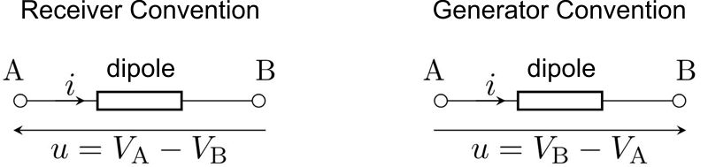
The two conventions encountered in electrodynamics.

In this chapter, we limit our discussion to the study of electrodynamic dipoles whose relationship between u and I is either linear or affine (i = a × u + b). Indeed, the primary objective is to become familiar with the solution methods.

Source: FEMTO, Les cours de physique. License CC BY-NC 4.0. Translated and adapted by Nicolae Sfetcu